> For the complete documentation index, see [llms.txt](https://aye10032.gitbook.io/prml-note/llms.txt). Markdown versions of documentation pages are available by appending `.md` to page URLs; this page is available as [Markdown](https://aye10032.gitbook.io/prml-note/di-er-zhang-sheng-cheng-shi-fen-lei-qi/2.3-jun-zhi-xiang-liang-he-xie-fang-cha-ju-zhen-de-can-shu-gu-ji.md).

# 2.3 均值向量和协方差矩阵的参数估计

* 在贝叶斯分类器中，构造分类器需要知道类概率密度函数$$p(x|\omega\_i)$$
* 如果按先验知识已知其分布，则只需知道分布的参数即可
  * 例如：类概率密度是正态分布，它完全由其均值向量和协方差矩阵所确定

对均值向量和协方差矩阵的估计即为贝叶斯分类器中的一种<mark style="color:orange;">**参数估计**</mark>问题

{% hint style="success" %}
**参数估计的两种方式**

* 一种是将参数作为非随机变量来处理，例如<mark style="color:purple;">**矩估计**</mark>就是一种非随机参数的估计
* 另一种是随机参数的估计，即**把这些参数看成是随机变量**，例如<mark style="color:purple;">**贝叶斯参数估计**</mark>
  {% endhint %}

## 2.3.1 定义

### 均值

设模式的概率密度函数为$$p(x)$$，则均值的定义为：

$$
m = E(x) = \int\_x xp(x)dx
$$

其中，$$x=(x\_1,x\_2,\dots,x\_n)^T$$，$$m=(m\_1,m\_2,\dots,m\_n)^T$$

由大数定律有，均值的估计量为：

$$
\hat{m} = \frac{1}{N}\sum^N\_{j=1}x\_j
$$

### 协方差

协方差矩阵为：

$$
C= \begin{pmatrix} c\_{11} & c\_{12} & \cdots & c\_{1n}\ c\_{21} & c\_{22} & \cdots & c\_{2n}\ \vdots & \vdots & \ddots & \vdots\ c\_{n1} & c\_{n2} & \cdots & c\_{nn} \end{pmatrix}
$$

其中，每个元素的定义为：

$$
\begin{align} c\_{ij} &= E{(x\_i-m\_i)(x\_j-m\_j)} \nonumber \ &=\int\_{-\infty}^{\infty}\int\_{-\infty}^{\infty}(x\_i-m\_i)(x\_j-m\_j)p(x\_i,x\_j)dx\_idx\_j \nonumber \end{align}
$$

其中，$$x\_i$$、$$x\_j$$和$$m\_i$$、$$m\_j$$分别为**x**、**m**的第i和j个分量。

将协方差矩阵写成向量的方式为：

$$
\begin{align} C&=E{(x-m)(x-m)^T} \nonumber \ &=E{xx^T} - mm^T \nonumber \end{align}
$$

则根据大数定律，协方差的估计量可以写为：

$$
\hat{C} \approx \frac{1}{N}\sum^{N}\_{k=1}(x\_k-\hat{m})(x\_k-\hat{m})^T
$$

## 2.3.2 迭代运算

### 均值

假设已经计算了N个样本的均值估计量，此时若新增一个样本，则新的估计量为：

$$
\begin{align} \hat{m}(N+1) &= \frac{1}{N+1}\sum^{N+1}*{j=1}x\_j \nonumber \ &= \frac{1}{N+1}\left\[\sum*{j=1}^Nx\_j + x\_{N+1}\right] \nonumber \ &= \frac{1}{N+1}\[N\hat{m}(N) + x\_{N+1}] \end{align}
$$

迭代的初始化取$$\hat{m}(1)=x\_1$$

### 协方差

协方差与均值类似，当前已知

$$
\hat{C}(N)=\frac{1}{N}\sum^N\_{j=1}x\_jx\_j^T - \hat{m}(N)\hat{m}^T(N)
$$

则新加入一个样本后：

$$
\begin{align} \hat{C}(N+1) &= \frac{1}{N+1}\sum^{N+1}*{j=1}x\_jx\_j^T - \hat{m}(N+1)\hat{m}^T(N+1) \nonumber \ &= \frac{1}{N+1}\left\[\sum*{j=1}^Nx\_jx\_j^T + x\_{N+1}x\_{N+1}^T\right] - \hat{m}(N+1)\hat{m}^T(N+1) \nonumber \ &=\frac{1}{N+1}\[N\hat{C}(N) + N\hat{m}(N)\hat{m}^T(N) + x\_{N+1}x\_{N+1}^T] - \nonumber \ &\ \frac{1}{(N+1)^2}\[N\hat{m}(N) + x\_{N+1}]\[N\hat{m}(N) + x\_{N+1}]^T \end{align}
$$

由于$$\hat{m}(1)=x\_1$$，因此有$$\hat{C}(1) = 0$$

## 2.3.4 贝叶斯学习

* 将概率密度函数的参数估计量看成是随机变量$$\theta$$，它可以是纯量、向量或矩阵
* 按这些估计量统计特性的先验知识，可以先粗略地预选出它们的密度函数
* 通过训练模式样本集$${x\_i}$$，利用贝叶斯公式设计一个迭代运算过程求出参数的后验概率密度$$p(\theta|x\_i)$$
* 当后验概率密度函数中的随机变量$$\theta$$的确定性提高时，可获得较准确的估计量

具体而言，就是：

$$
p(\theta|x\_1,\cdots,x\_N) = \frac{p(x\_N|\theta,x\_1,\cdots,x\_{N-1})p(\theta|x\_1,\cdots,x\_{N-1})}{p(x\_N|x\_1,\cdots,x\_{N-1})}
$$

其中，<mark style="color:orange;">**先验概率**</mark>$$p(\theta|x\_1,\cdots,x\_{N-1})$$由迭代计算而来，而<mark style="color:orange;">**全概率**</mark>则由以下方式计算：

$$
p(x\_N|x\_1,\cdots,x\_{N-1})=\int\_xp(x\_N|\theta,x\_1,\cdots,x\_{N-1})p(\theta|x\_1,\cdots,x\_{N-1})d\theta
$$

因此，实际上需要知道的就是初始的$$p(\theta)$$

### 单变量正态密度的均值学习

{% hint style="info" %}
假设有一个模式样本集，其概率密度函数是单变量正态分布$$N(\theta,\sigma^2)$$，均值$$\theta$$待求，即：

$$
p(x|\theta)=\frac{1}{\sqrt{2\pi}\sigma}\exp{\left\[-\frac{1}{2}\left(\frac{x-\theta}{\sigma^2}\right)^2\right]}
$$

给出N个训练样本$${x\_1,x\_2,\dots,x\_N}$$，用贝叶斯学习计算其均值估计量。

对于初始条件，设 $$p(\theta)=N(\theta\_0,\sigma^2\_0)$$，$$p(x\_1|\theta)=N(\theta,\sigma^2)$$，由贝叶斯公式可得：

$$
\begin{align} p(\theta|x\_1) &= a\cdot p(x\_1|\theta)p(\theta)\nonumber \ &= a\cdot \frac{1}{\sqrt{2\pi}\sigma}\exp{\left\[-\frac{1}{2}\left(\frac{x-\theta}{\sigma^2}\right)^2\right]}\cdot \frac{1}{\sqrt{2\pi}\sigma\_0}\exp{\left\[-\frac{1}{2}\left(\frac{x-\theta\_0}{\sigma\_0^2}\right)^2\right]}\nonumber \end{align}
$$

其中a是一定值。由贝叶斯法则有：

$$
p(\theta|x\_1,\dots,x\_N)=\frac{p(x\_1,\dots,x\_N|\theta)p(\theta)}{\int\_\varphi p(x\_1,\dots,x\_N|\theta)p(\theta)d\theta}
$$

此处$$\phi$$表示整个模式空间，由于每一次迭代是逐个从样本子集中抽取，因此N次运算是<mark style="color:orange;">**独立的**</mark>，上式由此可以写成：

$$
\begin{align} p(\theta|x\_1,\dots,x\_N)&=a\cdot\left{\prod\_{k=1}^Np(x\_k|\theta)\right}p(\theta)\nonumber \ &=a\cdot\left{\prod\_{k=1}^N\frac{1}{\sqrt{2\pi}\sigma}\exp{\left\[-\frac{1}{2}\left(\frac{x\_k-\theta}{\sigma^2}\right)^2\right]}\right}\cdot\frac{1}{\sqrt{2\pi}\sigma\_0}\exp{\left\[-\frac{1}{2}\left(\frac{x-\theta\_0}{\sigma\_0^2}\right)^2\right]}\nonumber \ &=a^{'}\exp{\left\[-\frac{1}{2}\left{\sum\_{k=1}^N\left(\frac{x\_k-\theta}{\sigma}\right)^2\right} + \left(\frac{x-\theta\_0}{\sigma\_0^2}\right)^2\right]}\nonumber \ &= a^{\prime \prime} \exp \left\[-\frac{1}{2}\left{\left(\frac{N}{\sigma^2}+\frac{1}{\sigma\_0^2}\right) \theta^2-2\left(\frac{1}{\sigma^2} \sum\_{k=1}^N x\_k+\frac{\theta\_0}{\sigma\_0^2}\right) \theta\right}\right]\nonumber \end{align}
$$

将上式中所有与$$\theta$$无关的变量并入常数项$$a^{'}$$和$$a^{''}$$，则$$p(\theta|x\_1,\dots,x\_N)$$是$$\theta$$平方函数的指数集合，仍是<mark style="color:orange;">**正态密度函数**</mark>，写为$$N(\theta\_N,\sigma\_N^2)$$的形式，有：

$$
\begin{align} p(\theta|x\_1,\dots,x\_N) &= \frac{1}{\sqrt{2\pi}\sigma\_N}\exp{\left\[-\frac{1}{2}\left(\frac{\theta-\theta\_N}{\sigma\_N}\right)^2\right]}\nonumber \ &= a^{'''}\exp{\left\[-\frac{1}{2}\left(\frac{\theta^2}{\sigma^2\_N}-2\frac{\theta\_N\theta}{\sigma^2\_N}\right)\right]}\nonumber \end{align}
$$

上述两式相比较，可得：

$$
\begin{align} \frac{1}{\sigma^2}&=\frac{N}{\sigma^2} + \frac{1}{\sigma^2\_0}\nonumber \ \frac{\theta\_N}{\sigma\_N^2} &= \frac{1}{\sigma^2}\sum^N\_{k=1}x\_k + \frac{\theta\_0}{\sigma\_0^2}\nonumber \ &= \frac{N}{\sigma^2}\hat{m} + \frac{\theta\_0}{\sigma\_0^2}\nonumber \end{align}
$$

解出$$\theta\_N$$和$$\sigma\_N$$，得：

$$
\begin{align} \theta\_N &= \frac{N\sigma\_0^2}{N\sigma\_0^2 + \sigma^2}\hat{m}\_N + \frac{\sigma^2}{N\sigma\_0^2 + \sigma^2}\nonumber \ \sigma\_N^2 &= \frac{\sigma\_0^2\sigma^2}{N\sigma\_0^2 + \sigma^2}\nonumber \end{align}
$$

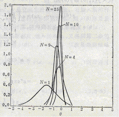
即根据对样本的观测，求得均值$$\theta$$的<mark style="color:purple;">**后验概率密度**</mark>$$p(\theta|x\_i)$$为$$N(\theta\_N,\sigma\_N^2)$$，其中：

$$\theta\_N$$是先验信息（$$\theta\_0,\sigma\_0^2,\sigma^2$$）与训练样本所给信息（$$N,\hat{m}$$）适当结合的结果，是N个训练样本对均值的<mark style="color:purple;">**先验估计**</mark>$$\theta\_0$$的补充

$$\sigma\_N^2$$是<mark style="color:orange;">**对这个估计的不确定性的度量**</mark>，随着N的增加而减少，因此当$$N\to\infin$$时，$$\sigma\_N \to 0$$，代入上式可知只要$$\sigma\_0\neq0$$，则当N数量足够大时，$$\theta\_N$$趋于样本均值的估计量$$\hat{m}$$

<img src="https://4038108263-files.gitbook.io/~/files/v0/b/gitbook-x-prod.appspot.com/o/spaces%2FQvX394T4tC7TQRUQRFUu%2Fuploads%2Fgit-blob-7d7a36e0d2de5245fb80ea87fdb4cd1623ce64a3%2F2.3.1.png?alt=media" alt="" data-size="original">
{% endhint %}